Polynomial Functions Graphs: How to Read Zeros and Shape
Polynomial Functions Graphs made simple: read end behavior, zeros, multiplicity and shifts with plain examples you can sketch yourself.
You've factored the equation, drawn your axes, and stopped with your pencil in the air. Should the curve cross at that zero or bounce? Does the left side go up or down? And how much of the middle can you draw without calculating a whole page of points?
When you're studying polynomial functions graphs, the useful habit is to read ordered clues: ends, zeros, then turns. Each clue comes from the formula, so you can justify your sketch instead of hoping it looks familiar. You also need to know what the picture leaves out, because a small graphing window and a real-number axis can both hide solutions.
Read the Ends Before You Plot Anything
End behavior by degree and leading coefficient
| Degree and leading coefficient | Left end | Right end | Example |
|---|---|---|---|
| Even degree, positive leading coefficient | Rises | Rises | y = x² − 4 |
| Even degree, negative leading coefficient | Falls | Falls | y = −x² + 3 |
| Odd degree, positive leading coefficient | Falls | Rises | y = x³ − x |
| Odd degree, negative leading coefficient | Rises | Falls | y = −x³ + 2x |
The ends set the sketch's outer boundaries before you place its bends. They do not show where every turn belongs, but they keep the curve pointed in the right directions.
The degree is the highest exponent after like terms are combined. The leading coefficient is the number multiplying that highest power. Together, they determine the graph's behavior far to the left and far to the right.
Why the highest power controls the ends
For large positive or negative inputs, the highest-power term eventually outweighs the lower-power terms. In y = x³ − x, the −x term affects the middle, while x³ determines the distant ends.
An even power gives a positive result for either a positive or negative nonzero input. An odd power keeps the input's sign. A negative leading coefficient reverses the resulting directions, which accounts for each row in the table.
A rising left end climbs as you move farther left along the x-axis.
Find the leading term without unnecessary expansion
Consider this worked example:
y = (x − 1)(x + 2)(x − 5)
Multiplying the first two factors gives x² + x − 2. Multiplying that result by the remaining factor gives:
y = x³ − 4x² − 7x + 10
The leading term is x³, so the degree is 3 and the leading coefficient is positive. The graph falls on the left and rises on the right.
You can find the leading term directly by multiplying the highest-power part of each factor: x × x × x. Expanding the whole expression is unnecessary when you only need the end directions.
Checkpoint: Name the degree, identify the leading sign, and mark the end directions before plotting the zeros.
These directions describe what happens far from the origin. A short viewing window may show a local dip or rise before the graph reaches its eventual end behavior.
Finding Zeros and How the Graph Behaves at Each One
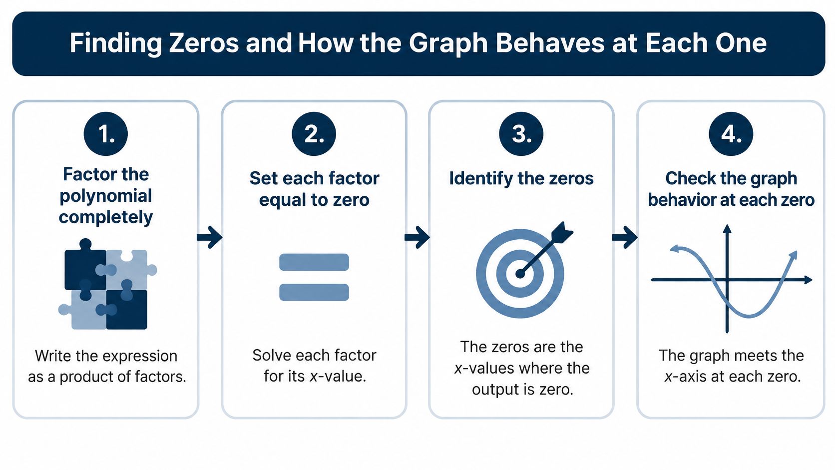
A zero gives you an exact place to start sketching near the x-axis. Factor the polynomial, set each factor equal to zero, and solve. Each solution is an input value; the corresponding x-intercept is the coordinate pair ((r, 0)). Record how many times each factor appears, since that multiplicity determines whether the curve crosses or touches the axis.
How multiplicity changes the graph at a zero
| Multiplicity | Behavior at the zero | Example factor | Look of the curve |
|---|---|---|---|
| 1 (odd) | Crosses the x-axis | (x − 2) | Crosses without flattening |
| 2 (even) | Touches the x-axis and turns back | (x + 1)² | Turns back at the axis |
| 3 (odd) | Crosses the x-axis, flatter at the zero | (x − 4)³ | Flattens as it crosses |
| 4 (even) | Touches the x-axis and turns back, flatter | (x + 3)⁴ | Flattens as it turns back |
Work from factors to intercepts
For y = (x + 1)²(x − 3), setting (x + 1 = 0) gives x = −1, with multiplicity 2. Setting (x − 3 = 0) gives x = 3, with multiplicity 1.
The graph touches the axis at ((-1, 0)) and crosses it at ((3, 0)). Watch the sign in the factor: (x + 1) is zero at −1, not 1. Substitution confirms the result.
Why the crossing rule works
As the input passes through a zero, an odd power of its factor changes sign, while an even power keeps the same sign. The other factors remain nonzero nearby, so they do not change this local behavior. An odd multiplicity therefore means the output's sign flips at that zero; an even multiplicity means it stays the same.
Polynomial graphs are smooth, so the curve bends gently through the axis instead of forming a corner. Higher multiplicity makes the graph flatter near the zero. A multiplicity of 1 crosses without that extra flattening.
If factoring stalls, the rational root test can suggest rational candidates when the coefficients are integers. A graphing tool can estimate real zeros, but an approximate picture alone may not establish exact multiplicity. Check repeated factors algebraically where possible, then mark each zero and use its multiplicity to determine the curve's behavior.
Count the multiplicity before drawing the curve at each zero.
Turning Points and What the Graph Hides
A degree-four polynomial can change direction at most three times. In general, a polynomial of degree n has at most n − 1 turning points, though its graph may have fewer. A turning point is where the curve changes direction, from rising to falling or the reverse.
The y-intercept gives another exact clue. For y = x³ − x, substituting x = 0 gives y = 0, so the graph passes through the origin. This point anchors the sketch without requiring you to locate a peak or valley.
A missing intercept may be outside the window
Suppose a polynomial has a real zero at x = 12, while the graphing window runs from −1 to 5. The intercept lies beyond the displayed range, so it cannot appear on the screen.
Widen the horizontal range before deciding that an expected zero is missing. Adjust the vertical range as well: a tall peak can compress nearby features until they are hard to inspect.
| What you notice | What to check |
|---|---|
| An expected real intercept isn't visible | Horizontal window boundaries |
| A touch looks like a crossing | Local zoom and the factor's multiplicity |
| Fewer intercepts appear than the degree suggests | Repeated roots and non-real roots |
Some roots don't belong on the real axis
The Fundamental Theorem of Algebra counts complex roots with multiplicity. A degree-three polynomial has three roots in that sense, but those roots need not produce three distinct x-intercepts. An educational analysis of real polynomials and complex roots discusses why a graph may show only some symbolic solutions and explores domain restrictions and interactive three-dimensional views.
For example, x² + 1 has no x-intercepts because its output is always positive for inputs. Its roots are i and −i, where i² = −1; these solutions do not lie on the number axis.
A root plot in the complex plane displays each solution by its real and imaginary parts. A polynomial graph instead displays real input-output pairs, so non-real roots are outside its view.
Ask of any graph: what does this picture fail to show?
Graphing a Polynomial Step by Step
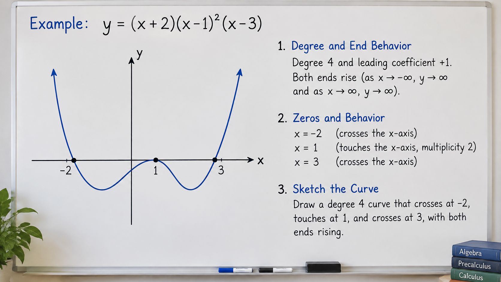
Use y = (x + 2)(x − 1)²(x − 3) as a complete worked example. Keep it in factored form, because that form makes the intercepts easier to read.
Use the labeled sketch below as a reminder to annotate your reasoning, not just your points.
Build the sketch from exact information
Identify the degree and leading coefficient. The leading product is x × x² × x = x⁴, giving degree 4 and leading coefficient +1. Mark both ends rising to avoid drawing the whole curve upside down.
Find the zeros: −2, 1, and 3. Their multiplicities are 1, 2, and 1, respectively, so label the outer intercepts “cross” and the middle intercept “touch.”
Calculate the y-intercept. Substituting x = 0 gives (2)(1)(−3) = −6, so the graph passes through (0, −6). This prevents a sketch that has correct zeros but floats on the wrong side of the axis.
Draw and label the axes, then plot (−2, 0), (1, 0), (3, 0), and (0, −6). Leave space above the axis for the rising ends and below it for the middle valleys.
Test the regions between zeros. At x = 0, the output is −6; at x = 2, it is (4)(1)(−1) = −4; at x = 4, it is (6)(9)(1) = 54. The curve is below the axis on both sides of the touch at x = 1, then above it beyond x = 3.
Sketch a smooth, connected curve through the marked points. Cross downward at −2, return to touch the axis from below at 1, dip again, and cross upward at 3 before continuing toward the rising right end.
Check the intervals, not just the dots
The sign tests guard against a tempting mistake: drawing a crossing at x = 1 because connecting dots feels easier that way. Both neighboring intervals have negative outputs, so that crossing would contradict the calculations.
For the untested region left of −2, all three displayed factors give a positive product: the outer factors are negative and the squared factor is positive. That agrees with the rising left end.
For a moving demonstration of the graphing process, use the video alongside your own annotated axes.
Your sanity check is specific: this degree-four sketch has no more than three turns. It stays below the axis between −2 and 3 except for the touch at x = 1, and it lies above the axis after 3.
You haven't calculated the exact valley locations, and that's fine for a qualitative sketch. Don't label an estimated turning point as exact.
Shifts, Stretches and Flips Explained
Each change to a polynomial moves or reshapes its graph in a predictable way. Track what happens to the inputs and outputs, and familiar features such as the vertex or zeros become useful checkpoints.
How each change transforms a polynomial graph
| Change | What it does | Example |
|---|---|---|
| f(x) + k | Shifts up by k when k is positive | y = x³ + 2 is y = x³ raised 2 units |
| f(x − h) | Shifts right by h when h is positive | y = (x − 3)² moves the vertex from 0 to 3 |
| −f(x) | Reflects across the x-axis | y = −x² opens downward |
| f(−x) | Reflects across the y-axis | y = (−x)³ = −x³ flips the odd-degree graph left to right |
| a f(x) with a greater than 1 | Stretches vertically | y = 3x² is steeper than y = x² |
| f(bx) with b greater than 1 | Compresses horizontally | y = (2x)² = 4x² is narrower than y = x² |
Shifts change where familiar features sit
Start with y = x³. Adding 2 outside the power increases every output by 2, so each point moves upward. The origin's image moves to (0, 2).
A change inside the function shifts the graph horizontally. For y = (x − 3)², the squared expression is zero at x = 3, so the vertex moves from (0, 0) to (3, 0). For an inside change, the shift runs opposite to the sign: (x − 3) moves the graph 3 units right.
Stretches change distances
Multiplying the whole function by a positive factor greater than 1 increases every vertical distance from the x-axis. Thus, y = 3x² has outputs three times those of y = x² at matching inputs, while its zero stays put.
Replacing x with bx, where b is greater than 1, compresses the graph horizontally. The same output as before now occurs at a smaller distance from the y-axis.
For the square function, (2x)² = 4x², so a horizontal compression also has a vertical-stretch description. This equivalence comes from the algebra of this particular function; the same multiplier need not describe other polynomials.
Reflections change orientation
A minus sign outside the function reverses the signs of its outputs, reflecting the graph across the x-axis. A minus sign inside reverses the input positions, reflecting it across the y-axis.
For x³, either reflection produces −x³. For x², reflection across the y-axis leaves the graph unchanged because (−x)² = x².
After a shift, recompute a zero to check its new position. Solving (x − 3)² = 0 gives x = 3, confirming the rightward move.
Justifying a Polynomial Graph and Checking Your Sketch
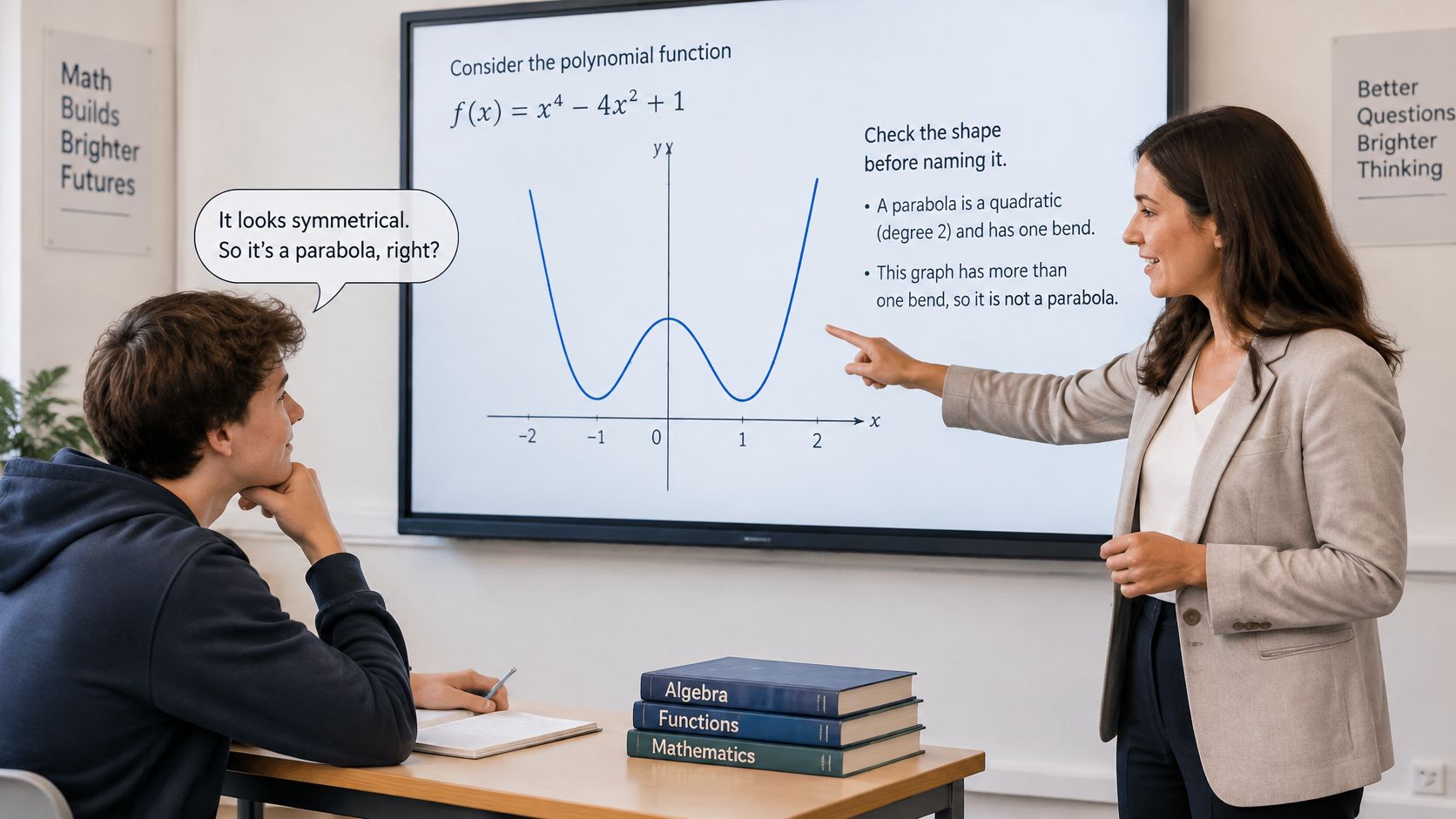
A learner sees a smooth curve with a wavy middle and calls it a parabola because it looks symmetrical. The observation about symmetry may be right, but the classification doesn't follow. Symmetry alone doesn't identify the degree or establish that a curve is quadratic.
An INDRUM proceedings study of secondary- and higher-education students found that some learners recognized polynomial graphs only when they resembled monomial graphs, relying on symmetry or the belief that an even-degree polynomial must be a parabola; in one unusual graph-identification task, 52% of high-school students and 35% of higher-education students gave at least one answer without justification. The useful response is to require reasons that another learner can check, rather than collect more familiar-looking pictures.
Same ends, different middle
Compare y = x² with y = x⁴ − 5x². Both have even degree, positive leading coefficients, and rising ends, but they don't have the same local structure.
The first is a monomial, a polynomial with a single term. The second is a sum of terms, and factoring gives:
y = x²(x² − 5) = x²(x − √5)(x + √5)
Its zeros are 0, with multiplicity 2, and −√5 and √5, each with multiplicity 1. It has three turning points, including a touch at the origin, so it isn't a parabola.
Notice that both examples are also symmetrical about the y-axis. Even correct observations can be insufficient evidence: matching ends and matching symmetry still leave important differences in roots and turns.
The classroom image below reflects the useful teaching habit: point to a feature, then connect it to a property of the formula.
Use evidence that can reject a wrong sketch
Apply these checks to a proposed match between formula and graph:
- Ends from the leading term. State the degree and leading sign, then compare them with the directions shown. Don't accept a matching middle if the distant directions contradict the formula.
- Axis behavior from the factors. Identify each real zero and its multiplicity. A correctly placed intercept can still be drawn incorrectly.
- Turns and the vertical anchor. Compare the number of turns with what the degree allows, and calculate the y-intercept. Passing these checks supports a sketch, although it doesn't prove every detail is exact.
Take a deliberately failing sketch of y = (x − 2)² that crosses the axis at x = 2. It may have rising ends and pass through the correct y-intercept, (0, 4), but it fails the axis-behavior check.
The factor has multiplicity two. More directly, a square cannot become negative, so a crossing into negative outputs is impossible. That's a justification, not a preference about how a parabola should look.
Make checking part of practice
Try three sketches per week on graph paper as a manageable practice routine, not a speed target. Annotate each with end arrows, multiplicities, and an exact y-intercept before comparing it with a graphing tool or additional test values.
If the display disagrees with your formula, inspect the window size before abandoning the mathematics. Then check your entry, expansion, factoring, and arithmetic; zooming won't repair an algebra error.
Choose one homework function now, run the three checks, and write one sentence per check stating the result. Your goal isn't a beautiful curve. It's a sketch whose important features you can explain.
Upfling lets educators upload graph worksheets, annotated images, PDFs, and static lesson pages to shareable URLs. Visit Upfling to publish a polynomial practice sheet and its worked solutions, then share the materials with your class or study group.